
Shotgun metagenomics: the species in your samples, and the genes they carry.
We sequence all the DNA in a sample, not just one marker gene. That names microbes down to species, shows which gene functions they carry and can turn percentages into cell counts.
Read everything, then sort it out.
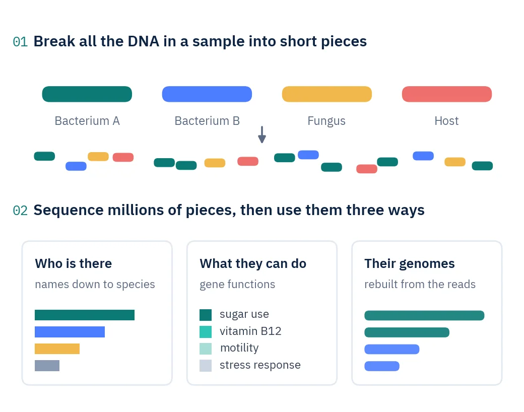
Shotgun sequencing breaks all the DNA in a sample into millions of short fragments and reads them at random. There is no primer and no marker gene, so bacteria, archaea, fungi and DNA viruses all end up in the data, together with DNA from the host.
Each read is compared against reference databases of complete genomes to name the organism it came from. Because the reads cover whole genomes rather than a short marker, microbes can be named down to species.
The same reads answer more questions. Matched against catalogues of gene functions, they show what the community is equipped to do. Assembled into longer stretches and sorted by organism, they rebuild draft genomes of microbes that nobody has cultured.
Sequencing gives shares of reads. Adding a known number of spike-in cells to each sample before DNA extraction turns those shares into cells per gram.
Key terms
- Metagenome
- All the DNA from all the organisms in one sample, read together.
- Read pair
- Two short reads, 150 letters each, from the two ends of one DNA fragment.
- Host DNA
- DNA from the person, animal or plant the sample came from. It uses up sequencing depth.
- Taxonomic profile
- A list of the organisms in a sample and the share of reads each one gets.
- MAG
- A metagenome-assembled genome: a draft genome of one microbe rebuilt from a mixed sample.
- Spike-in control
- A known number of foreign cells added to a sample so that read shares can be turned into cell counts.
Bring the question. We design the experiment around it.
- Which species are more or less common in my treated group than in controls?
- Which gene functions does the community carry, and which differ between groups?
- Did the total number of bacteria per gram change, or only their proportions?
- Can I recover genomes of microbes that nobody has cultured?
Where it is used
- Gut microbiome cohortsSpecies-level profiles across patients, diets and time points.
- Treatment and intervention studiesWhich species and gene functions shift after a drug, probiotic or diet.
- Diet and host from faecal DNAWhich host species and which plant families show up in faecal samples.
- Environmental samplesSoil, sediment, water and surfaces, including organisms that cannot be cultured.
- Samples with very little DNACleanroom swabs and other low-biomass material.
- Absolute microbial loadCells per gram, when you need to know whether bacteria truly grew or declined.
Four steps from sample to figures.
- Step 1
Plan depth and controls
We set the sequencing depth for your sample type, since host-rich samples need more reads, and decide whether spike-in controls are needed.
- Step 2
Check the DNA
Every sample is checked before library preparation, so problems show up while they are still cheap to fix.
- Step 3
Sequence
All the DNA is fragmented and sequenced as 150-letter read pairs.
- Step 4
Analyse and report
Species profiles, diversity and group comparisons, plus gene functions and genomes when the question needs them, with figures and a Methods section.
What the analysis shows you.
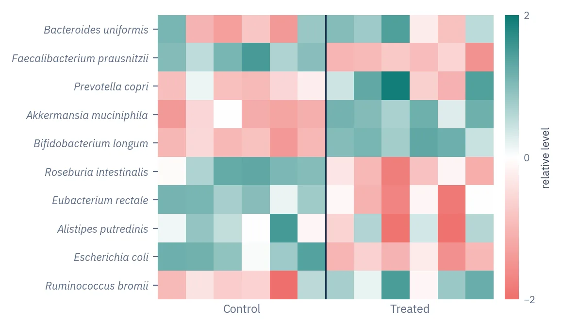
Species across samples
Each row is a species, each column a sample. Teal means more than that species’ average, coral means less, so group differences stand out.
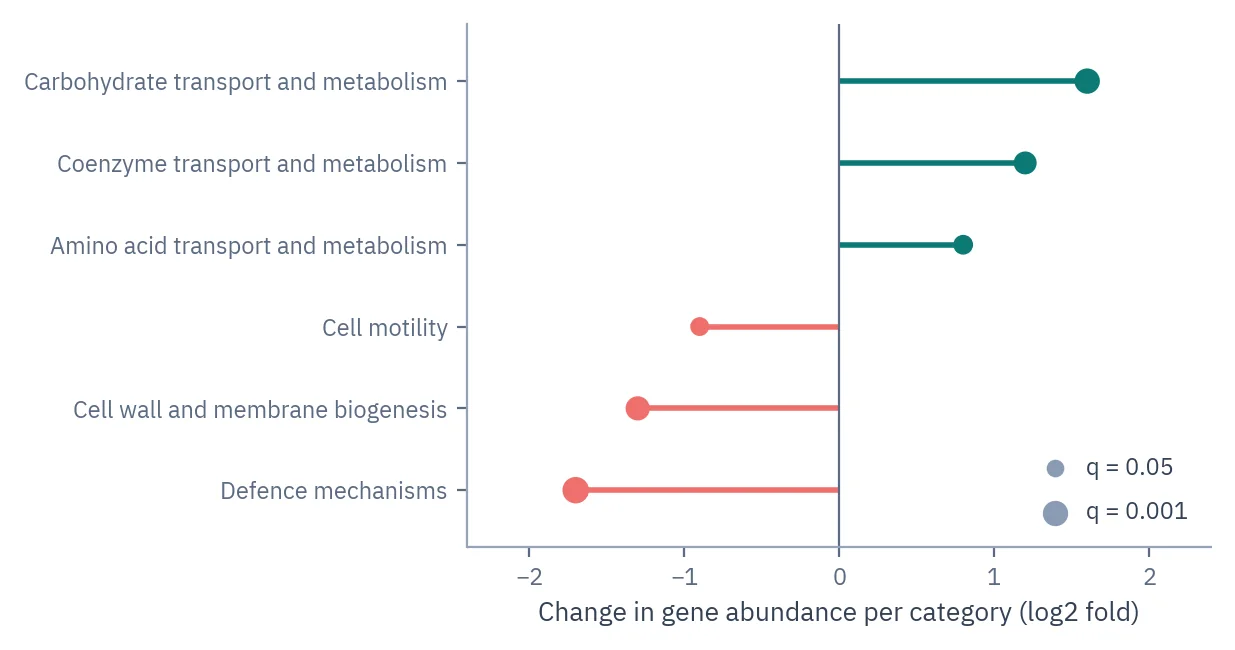
Gene functions that changed
Genes grouped into function categories and compared between groups. Bigger dots mean stronger statistical evidence.
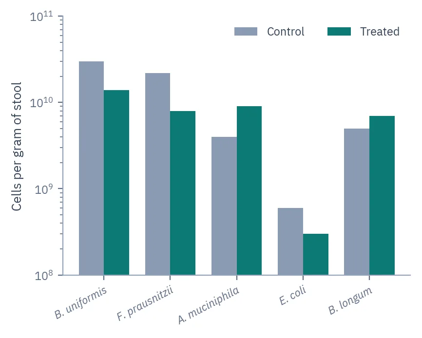
Cells per gram
Spike-in controls turn read shares into cell counts, so you see whether a microbe truly declined or only looks smaller because others grew.
Included as standard every project
- Quality filteringLow-quality bases and adapter sequence are removed before analysis.
- Species-level profilesEvery read is matched against reference genomes, and abundances are estimated down to species.
- Composition tables at every levelCounts and shares from kingdom to species, as spreadsheets and charts.
- Diversity and community mapRichness per sample, and a map of how similar samples are, with a test for group differences.
- Differential abundanceWhich species changed between groups, corrected for testing many at once.
Added for your question custom
- Gene functionsGenes matched to function catalogues (KEGG orthologs, COG categories) and compared between groups.
- Genomes from the mixtureDraft genomes rebuilt from the reads, checked for completeness and contamination, and named.
- Absolute countsSpike-in controls convert read shares into cells per gram.
- Host and dietHost species and diet plant families identified from faecal DNA.
- Confirmation of key hitsA second classification and a genome-coverage check show whether a flagged organism is really there.
- Resistance genes and strainsAntibiotic resistance genes, virulence factors and strain-level differences.
- Networks and predictionCo-occurrence networks and machine-learning classification of groups.
What goes in, and how we run it.
- Sequencing
- Illumina NovaSeq X Plus or NextSeq 2000, 150 bp read pairs
- Typical depth
- 10–20 million read pairs for stool · more for host-rich samples such as swabs and tissue
- Samples
- Stool, soil, sediment, water, swabs, tissue, cleanroom and low-biomass samples
- Input
- Extracted DNA or raw samples · low-input samples accepted
- Cell counts
- Spike-in controls added before DNA extraction, on request
- Main tools
- Kraken2, Bracken, MEGAHIT, CheckM2, GTDB-Tk, eggNOG
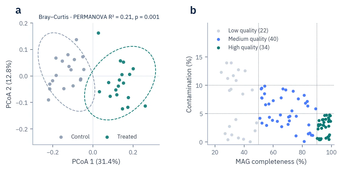
Figures, interpretation and Methods, ready for the manuscript.
- ReportInterpretation written against your hypothesis
- FiguresPublication-ready figures for the manuscript
- MethodsMaterials & Methods text for the paper
- Tables and dataAll results as tables, plus the processed data files
Shotgun or amplicon?
Send us the question and we recommend one, including when the cheaper option is enough.
| Aspect | Shotgun metagenomics | Amplicon sequencing |
|---|---|---|
| What is read | All DNA in the sample | One marker gene |
| Naming depth | Species | Usually genus |
| Function | Read from the genes themselves | Predicted from who is there |
| Extra outputs | Draft genomes, cell counts, host and diet | Fungi, protists and animals on their own markers |
| Best when | Genes, genomes or species-level detail matter | Many samples and a tight budget per sample |
Before you send samples
Related services
How deep should I sequence?
It depends on how much host DNA your samples contain. Stool is mostly microbial, so 10–20 million read pairs give species-level profiles. Swabs, saliva and tissue can be more than 90% host DNA and need more reads. We set the depth per sample type in the design review.
My samples contain a lot of host DNA. What happens?
Host reads are recognised as host DNA, so they are not mistaken for microbes. Because they still use up reads, host-rich samples are sequenced deeper.
Which organisms can shotgun detect?
Bacteria, archaea, fungi, protists and DNA viruses, all from the same data, because no marker gene or primer is involved.
Can you rebuild genomes from my samples?
Yes. Reads are assembled, sorted into draft genomes, checked for completeness and contamination, and named against a genome-based taxonomy.
Can I get absolute abundances instead of percentages?
Yes. A spike-in control with a known number of cells is added to each sample before DNA extraction, and we report cells per gram.
Will I learn what the community does?
You learn its genetic potential: which gene functions are present and how they differ between groups.
I already have shotgun data. Can you analyse it?
Yes. Send the raw FASTQ files or the accession number of a public dataset, with a sample sheet that lists the groups.
If something goes wrong on this project, you pay €0 to fix it.
- Sample problems €0
- Library prep redo €0
- Resequencing €0
- Reviewer re-analysis €0